Magnetic fields generated
by conducting lines

This section is an introduction to the theory of the magnetic field around a current carrying conducting line and the forces acting on a magnetic marker inside the produced magnetic gradient field. Additionally, some basic ideas about the manipulation and positioning of a magnetic markers with conducting lines will be discussed.

Figure 1.9: Magnetic fields of a rectilinear current, remade after [1]

[Magnetic field lines around a rectilinear current]         [Magnetic field at point $P$ produced by a rectilinear current]

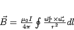
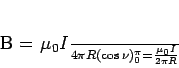
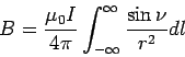
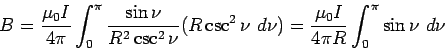
A straight current generates a magnetic field that is inverse proportional to the radius $R$. The field lines are concentric circles orthogonal to the straight current, see figure 1.9(a). To calculate the magnetic field of a straight current we start from the Ampère-Laplace law:

$$\vec{B} = \frac{\mu_0I}{4\pi} \oint \frac{\vec{u_T} \times \vec{u_r}}{r^2} dl$$ (1.2)

with the unit vectors $\vec{u_T}$ and $\vec{u_r}$, $\mu_0 = 4\pi\cdot 10^{-7} \frac{mkg}{C^2}$ and assuming a constant current density. As shown in figure 1.9(b), the vector $\vec{u_T} \times \vec{u_r}$ is for every point $P$ and every element $dl$ perpendicular to the plane which is determined by $P$ and the current $I$. Hence $\vec{u_T} \times \vec{u_r}$ equals $\vec{u_\nu}$. The magnetic field at point $P$, originating from $dl$, is tangent to the circle of radius $R$ that passes through $P$. It is centered on the current and it is in a plane perpendicular to the current. So, when we integrate equation 1.2 all contributions in the integral have the same direction $\vec{u_\nu}$, and the resultant magnetic field $\vec{B}$ is also tangent to the circle. Thus, it is only necessary to find the magnitude of $\vec{B}$. The magnitude of $\vec{u_T} \times \vec{u_r}$ is $\sin\nu$, because both vectors are unit vectors. Therefore, we get for the magnitude of a rectilinear current:

$$B = \frac{\mu_0I}{4\pi} \int_{-\infty}^{\infty} \frac{\sin\nu}{r^2} dl$$ (1.3)

It can be seen in figure 1.9(b) that $r = R \cos\nu$ and $l = -R \cot\nu$ thus $dl = R \frac{1}{\sin^2\nu}~d\nu = R \csc^2\nu~d\nu$. Hence we get

$$B = \frac{\mu_0I}{4\pi} \int_{0}^{\pi} \frac{\sin\nu}{R^2 \... ...\nu~d\nu) = \frac{\mu_0I}{4\pi R} \int_{0}^{\pi} \sin\nu~d\nu$$ (1.4)

With $l = -\infty$ corresponding to $\nu = 0$ and $l = +\infty$ corresponding to $\nu = \pi$ we get the law of Biot-Savart:

$$B = \frac{\mu_0I}{4\pi R}(\cos\nu)_0^\pi = \frac{\mu_0I}{2\pi R}$$ (1.5)

or in vector form

$$\vec{B} = \frac{\mu_0I}{2\pi R}\vec{u_\nu}$$ (1.6)

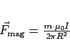
After we can calculate the magnetic field $B$ at every point around a long and thin conducting line, we also want to set a superparamagnetic marker inside this magnetic field and calculate the acting forces.

Figure 1.10: Sketch of a simple setup to manipulate a magnetic marker with a conducting line on a surface.

0.5

Figure 1.10 shows a simplistic setup for a magnetic particle on a surface near a conducting line. When we neglect different heights of the center of the magnetic particle and the center of the conducting line, this is only a two-dimensional problem. While the current flows in-plane
through the conducting line, the magnetic field is always perpendicular to the plane and so it is easy to calculate the magnetic field for every point in the plane. When the current is turned on in this simple setup, a magnetic field is generated that affects the magnetic particle. In the case of ferromagnetic markers with large anisotropy, the markers would start to rotate in order to align themselves to the magnetic field, as the dipole wants to go into the state of minimal energy [29]. The magnetic torque forced on the marker is $\vec{\tau} = \vec{m} \times \vec{B}$.

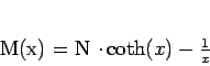
But in this thesis, only superparamagnetic markers were used. The ferromagnetic crystallites inside the core of the markers are so small ($\approx$1-10nm) that they show superparamagnetic behaviour. In such small crystallites, the thermal energy is sufficient to change the direction of the magnetisation, so the overall magnetic moment averages to zero. Therefore, the crystallite exhibits a behaviour similar to paramagnetism, where the magnetic moment $M$ follows the langevin equation:

$$M(x) = N \cdot \coth(x) - \frac{1}{x}$$ (1.7)

with $x = \frac{\mu_0 H}{k_B T}$. In an outer magnetic field, the magnetic moment in the crystallite instantaneously aligns to the outer magnetic field, and, therefore, generates an own outer magnetic field. The net magnetic field of the superparamagnetic markers increases with a higher outer field until all magnetic moments are aligned, and the magnetic moment is saturated. So, in a magnetic gradient field, as generated by the conducting line, the markers additionally feel a translational force $\vec{F}_{\rm mag}$ in the direction of the magnetic gradient.

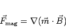
The change of the magnetic moment of the markers is very small for the applied outer fields. Therefore, it is only a small error when we assume the marker as a constant magnetic dipole for the bond-force measurements (see chapter 4). The force exerted on the marker can then be written as [71]:

$$\vec{F}_{\rm mag} = \nabla(\vec{m}\cdot\vec{B})$$ (1.8)

With the assumption that the magnetic dipole moment instantly aligns to the outer magnetic field and the particle adheres to the surface in the same position, the vector product reduces to a scalar product. The magnetic force can then be written as:

$$\vec{F}_{\rm mag} = \vert\vec{m}\vert\nabla\vert\vec{B}\vert = m\cdot \frac{dB}{dR}$$ (1.9)

Together with equation 1.5 we get:

$$\vec{F}_{\rm mag} = \frac{m \cdot \mu_0 I}{2\pi R^2}$$ (1.10)

To hold a particle in a specified position, a trap must be build with the magnetic fields. But according to EARNSHAWS theorem, it is not possible to build a trap with any combinations of outer magnetic fields. SAMUEL EARNSHAW already proved in 1842 [36] that if inverse-square-law forces, such as the magnetic force $\vec{F}_{\rm mag}$, govern a group of charged particles, they can never be in stable equilibrium. The reason for this is that inverse-square-law forces follow the Laplace partial differential equation, and the solution of this equation does not have any local maxima or minima. There are only saddle-type equilibrium points, instead. Although not applicable for the experiments in this thesis, in principle one can circumvent Earnshaw's theorem by using time-varying fields, active-feedback systems, diamagnetic systems (extremely low forces) or superconductors.

Naturally one would like to guide a particle between the conducting lines that create the magnetic field. But this is only possible for particles that follow the magnetic gradient to local minima. This was e.g. done by DEKKER et al.  [30] to guide neutral atoms on a chip. But the magnetic particles used in this thesis follow the magnetic gradient to the local maxima, and the local maxima are always at the edges and in the corners of the conducting lines.

So, in the experiments in this thesis, we trapped particles at the crossing of two conducting lines or in a corner (see chapters 3 and 5).